Where’s my point?

A reoccurring problem in computer vision has to do with finding the precise location of an object in the image. In this post, I want to discuss specifically the problem of finding the location of a blob or a point in an image. This is what you’d get when a light source is imaged.

Finding the center of the blob is a question I love asking in job interviews. It’s simple, can be solved with good intuition and without prior knowledge, and it shows a lot about how one grasps the process of image formation.

What’s a blob?

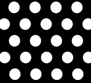
A blob is what’s formed on an image plane when imaging a light source. For instance, here’s how you might imagine a set of LEDs would appear in an image:

This is interesting problem because if we know the location of the center of each blob, and if we know the 3D pattern that generated it (eg. the 3D shape of the LED array) then we can reconstruct its position in 3D space.

There are many possible approaches here. Most of them are either too expensive computationally, unnecessarily complex or plainly inaccurate. Let’s discuss a few:

I) Averaging

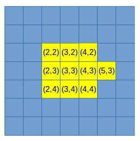
This one is rather simple. We take all the pixels associated with a blob and find their average. Here are two examples:

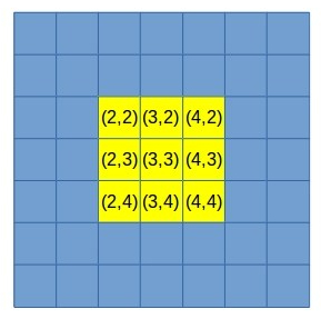
Computing the average of all pixels above would give us x=3 and y=3 as the sum of all x coordinates and all y coordinates is 27 and there are 9 pixels.

Here, however, the average is different. Now the average x is 3.2 and the average y is still 3. This isn’t surprising — the center is shifting to the right because of the additional pixel.

This computation is simple and require very little computation. However, it’s obviously not very precise. We can easily see that our average is in the space of 1/2 pixel — the center either lands on a pixel center or its edge (between two pixels). This is terrible accuracy for 3D reconstruction (unless you have a super narrow field of view and/or extremely high resolution image sensor).

But wait, it gets worse. This method doesn’t take into account the brightness of pixels. For example, imagine pixel (5,3) above was extremely dim. So dim, in fact, that it would be just on the threshold of our image sensor. The result will be that the pixel would appear or disappear in consecutive frames due to image noise. The center of the blob will be greatly effected by this phenomena. Not good.

II) Circle Fit

How about fitting a circle to the blob? It seems like this would give us much higher precision and aren’t circles pretty robust to noise?

Well yes in theory but not so much in practice.

First, let’s consider the image of even a really small light source. The light source isn’t going to be a point source in practice. We can imagine it has some small circular shape. But, when that light source gets projected onto the image plane, the result is an ellipse and not a circle. Fitting an ellipse is much more complex and less robust than circle fit.

Second, the image formation process is unlikely to result in pixels that are all saturated. We are going to get shades of white as the distance from the true center increases. Here’s an example:

As can be seen in the image, pixels have less brightness when further out from the blob center. In fact, pixels at the edge of the blob might not always pass the sensor’s threshold and remain black. These pixels are going to have a significant impact on the fit.

And finally, in many cases blobs are going to be pretty small. Circle fit is much less robust with fewer pixels.

Weighted Average

A weighted average is almost as simple as the averaging method discussed above. However, it takes into account the strength of the signal in each pixel and it doesn’t assume the projected shape is a circle. Weighted average takes the brightness level of each pixel, and uses it as a weight for the average.

Now, imagine the 2nd example above, where all pixels have brightness level of 255, except for pixel (5,3) that is very dim, say brightness level of 10. Now, our weighted average will yield: x = 3.008 while y remains 3. This makes perfect sense: the dim pixel is pulling the center only slightly towards it. If that pixel was brighter, the pull would be stronger and the computed center will shift towards it.

Weighted average is also a great way to eliminate noise in the image. It’s simple, precise and much more robust.

Summary

I’ve used this method to solve multiple computer vision problems over time. Check out my patents page. Some of them use a version of this technique.

Position Tracking for Virtual Reality

I developed the original position tracking for the Oculus Rift headset and controllers.
In this post, I will discuss why position tracking is important for Virtual Reality and how we realized it at Oculus.

What is Position Tracking?

Position tracking in the context of VR is about tracking the user’s head motion in 6D. That is, we want to know the user’s head position and orientation. Ultimately, we will expand this requirement to tracking other objects / devices such as controllers or hands. But for now, I’ll focus on head motion.

Tracking the head let’s us render the right content for the user. For instance, as you move your head forward, you expect the 3D virtual world to change: objects will get closer to you, certain object will go out of the field of view, etc. Similarly, when you turn around, you expect to see what was previously behind you.

Virtual reality can cause motion sickness. If the position and orientation updates are wrong, shaky or just imprecise, our brain will sense the conflict between proprioception and vision — we know how the head, neck and body is moving, and we know what we expect to see, the mismatch causes discomfort.

To give you a sense of the requirements: we’re looking for a mean precision of about 0.05[mm] and a latency of about 1[ms]. In the case of a consumer electronics device, we also want to system cost to be low in $ and computation.

Note: the following assumes tracking of a single headset using a single camera. Mathematically, using stereo is easier. However, the associated cost in manufacturing and calibration are significant.

Basic Math

We can compute the pose of an object if we know its structure. In fact, we need as few as 3 points to compute a 6D pose:

If we know the distance between P1, P2 and P3 in metric units and the camera properties (intrinsics), we can compute the pose of the object (P1,P2,P3) that creates the projection (p1,p2,p3).

There are just two hurdles:
(1) we need to be able to tell which point P(i) corresponds to a projected point p(j)
(2) in the above formulation, there can actually be more than one solution (pose) that creates the same projection

Here’s an illustration of #2:

ID’ing points

There are many ways to solve #1. For instance, we could color code the points so they are easy to identify. At Oculus we created the points using infra red LEDs on the headset. We used modulation — each LED switched between high and low — to create a unique sequence.

Later on, we were able to make the computation efficient enough that we didn’t need modulation. But that’s for another post 🙂

Dealing with multiple solutions

There are two primary ways to handle multiple solutions. First, we have many LEDs on the headset. This means that we can create many pose theories for subsets of 3 points. We expect the right pose to explain all of them. Second, we are going to track the pose of the headset over time — the wrong solution will make tracking break in the next few frames because while the right answer will change smoothly from frame to frame, the alternative pose solution will jump around erratically.

Tracking

Many problems in computer vision can be solved by either tracking or re-identification. Simply put, you can either use the temporal correlation between solutions or recompute the solution from scratch every frame.

Usually, taking advantage of the temporal correlation leads to significant computational savings and robustness to noise. However, the downside is that we end up with a more complex software: we use a “from scratch” solution for the first frame and a tracking solution for the following frames. When you design a real time computer vision system, you often have to balance the trade-off between the two options.

The Oculus’ position tracking solution uses tracking. We compute the pose for frame i as discussed above, and then track the pose of the headset in the following frames. When we compute the pose in frame n, we know where the headset was in frame n-1 and n-2. This means that not only we have a good guess for the solution (close to where it was in the previous frame), but we also know the linear and angular velocities of the headset.

The following illustration shows the process of refining the pose of the headset based on temporal correlation. We can make a guess for the pose of the headset (the blue point). We then compute where the projected LEDs should be in the image given that pose. Of course, there are going to be some errors — we can now adjust the pose locally to get the red solution below (the local minima).

Latency

So far so good — we have a clean solution to compute the pose of the headset over time using only vision data. Unfortunately, a reasonable camera runs at about 30[fps]. This means that we’re going to get pose measurements every 33[ms]. This is very far from the requirement of 1[ms] of latency…

Let me introduce you to the IMU (Inertial Measurement Unit). It’s a cheap little device that is part of every cellphone and tablet. It’s typically being used to determine the orientation of your phone. The IMU measures the linear acceleration and angular velocity. And, a typical IMU works at about 1[KHz].

Our next task, therefore, is to use the IMU together with vision observations to get pose estimation at 1[KHz]. This will satisfy our latency requirements.

Complementary Filter

The complementary filter is a well known method for integrating multiple sources of information. We are going to use it to both filter IMU measurements to track the orientation of the headset, and to fuse together vision and IMU data to get full 6D pose.

IMU: orientation

To compute the orientation of the headset from IMU measurements we need to know the direction of gravity. We can compute that from the acceleration measurements. The above figure shows we can do that by low-pass filtering the acceleration vector. As the headset moves around, the only constant acceleration the IMU senses is going to be gravity.

orientation = (orientation + gyro * dt) * (1 – gain) + accelerometer * gain

With knowledge of gravity, we can lock the orientation along two dimensions: tilt and roll. We can also estimate the change in yaw, but this degree of freedom is subject to drift and cannot be corrected with gravity. Fortunately, yaw drift is slow and can be corrected with vision measurements.

IMU: full 6D pose

The final step in our system integrates pose computed from the camera (vision) at a low frequency with IMU measurements at a high frequency.

err = camera_position – filter_position
filter_position += velocity * dt + err * gain1
velocity += (accelerometer + bias) * dt + err * gain2
bias += err * gain3

 

Summary

Now we have a fully integrated system that takes advantage of the advantages of the camera (position and no drift in yaw) and the IMU (high frequency orientation and knowledge of gravity).

The complementary filter is a simple solution that provides as with smooth pose tracking at a very low latency and with minimal computational cost.

Here’s a video of a presentation I gave together with Michael Abrash about VR at Carnegie Mellon University (CMU). In my part, I cover the position tracking system design.