Reinventing Food

The world is growing and faster than ever. Scientist predict we will cross 9B people this century. And while there are arguments about when that growth will stop and how quickly, one thing is clear: we are going to run out of food soon.

Recent research proposes that in order to accommodate such a large population, we are going to have to change our diet. Specifically, move away from meat and consume mostly (if not exclusively) fruit and vegetable.

Meat consumption has dire effects on the environment. It is expensive to grow, raises moral concerns, but primarily it is extremely ineffective. An average cow will consume 30 times more calories in its lifetime than it will provide. The number is much smaller (about 5 times) for poultry. And of course, the most effective way is to consume vegetable based calories.

The worldwide trend is clear: as countries get wealthier, their meat consumption increases. Together with the fact that the world’s population is larger than ever and growing, we are heading towards an environmental crisis and likely famine.

What can we do? Other than switching to a vegetarian diet, we also need to start thinking about optimizing our farming. This is where robotics, computer vision and machine learning can help. For example, fully automated farms that are controlled by algorithms can be extremely effective and minimize waste, space and therefore cost and environmental footprint.

Reconstructing a Room from a Single Image

I’ve bee involved in the current generation of Virtual Reality from early on. You can read more about that in my website [Dov Katz]. There are many exciting problems related to VR and computer vision but one that I always found exciting is that of reconstructing a room from a single image. All in all, humans seem to be pretty good at it. It is clear that we are good at estimating the true structure of a room because we have so much experience with rooms and the objects in it. Now, can machines do the same?

In a recent paper titled “LayoutNet: Reconstructing the 3D Room Layout from a Single RGB Image”  (you can read it here) the authors propose a deep learning architecture accompanied with a few computer vision techniques to reconstruct a room boundaries from a single image.

The idea is to first align the image with gravity so that floors are parallel to the ground and walls are perpendicular. This is done to reduce the complexity associated with tilted views. Then, Manhattan lines are computed and together with the images are fed into a CNN. The network returns corners and boundaries which are the building blocks of a 3D model for the room.

The final step is fitting surfaces to satisfy the corners and edges the network suggested. This completes a 3D model of the room. The results are actually quite good. Check out the video above to see some examples.

6D Pose Estimation using CNN

Tracking the 6D pose of an object is an important task with many applications. For example, it’s a key component for AR, VR and many robotics systems.

There are many approaches to solve this problem. For example, when you know something about the size of the object and trackable features on it. Or, when the tracked object is a moving camera (ie. SLAM). These techniques all rely on the stereoscopic vision principle (directly or indirectly). They basically relate multiple views to compute depth. The main issue with such methods is objects that are weakly textured, low resolution videos and low light conditions.

An alternative approach is using depth sensing data acquired by RGB-D cameras. Such solutions are quite reliable but expensive in power, cost, weight, etc. This makes them less than optimal for mobile devices.

People, however, seem to be able to determine the pose of an object effortlessly from a single image with no depth sensor. This is likely so because we have vast knowledge of object sizes and appearance. Which, of course, begs the question: can we estimate pose using machine learning?

In a recent paper, the authors propose an extension of YoLo to 3D. Yolo is a deep learning algorithm that detects objects by determining the correct 2D bounding box. Extending YoLo is therefore pretty straight forward. We want to learn the 2D corners of a projected 3D bounding box. If we can do that, reconstructing the 3D pose of the bounding box is simple.

The input to the system is a single-shot RGB image. The output is the object’s 6D pose. The proposed solution runs at an impressive 50 frames per second. This rate make it suitable for real time object tracking. The key component of this system is a new CNN architecture that directly predicts the 2D image locations of the projected vertices of the object’s 3D bounding box. The object’s 6D pose is then estimated using a PnP algorithm.

The authors show some impressive results. Here’s an image showing the computed bounding box for a few objects:

Experiencing real estate in 3D

When my wife Gili Katz and I were looking for a house, we would have loved to have the option to check out a few options in VR. You can check out my website (Dov Katz) for more info about Virtual Reality. Here’s about some recent development that make virtual real estate shopping a possibility:

Shopping for real estate can be quite frustrating. You need to search ads for what seems like the right place for you, then contact agents, schedule appointments, drive and finally walk-through the house for a few minutes. If it doesn’t seem very effective, it’s because it isn’t.

Fortunately, computer vision and Virtual Reality can save the day. Recently, a YC backed startup called “Send Reality” (send reality) developed a system that offers a full 3D-model of a real estate listing. With Send Reality, you can simply walk through a house in Virtual Reality.

Send Reality sends photographers out to the listed property. The photographer only needs to carry an iPad fitted with an off-the-shelf depth sensor. Send Reality’s application does the rest. The photographer walks through the property, snapping hundreds of thousands of photos. Next, the software stitches those photos together to create a complete 3D model of the property.

Send Reality claims to do the stitching particularly fast. They claim that “… what this means is that the 3D models we create are so much more realistic than anything else anyone else has made”. I’m not sure why the speed of stitching has anything to do with the quality of the model. However, being able to handle hundreds of thousands of photos certainly helps in creating a detailed 3D model.

The company is currently focusing on luxury residential markets. Websites listing such properties can now include a 3D tour of the properties. Early results indicate people spend much more time viewing a property when a 3D virtual tour is available. The cost of creating a 3D virtual tour of a single property is about $500.

While this technology is exciting, it seems like a problem that is already solved by Virtual Reality hardware manufacturer. For instance, Oculus’ Go device tracks the environment in much the same way Send Reality tracks it to build a 3D model. It wouldn’t be big step to add the automatic construction of such models to the device’s tracking system. And, of course, the potential of scanning and sharing 3D environments goes beyond real estate.

Semantic Adversarial Examples

Deep Neural Networks have enabled tremendous progress in computer vision. They help us solve many detection, recognition and classification tasks that seemed out of reach not too long ago. However, DNNs are known to be vulnerable to adversarial  examples. That is, one can tweak the input to mislead the network. For example, it is well documented that small perturbations can dramatically increase prediction errors. Of course, the resulting image looks like it was artificially manipulated and the process can be mitigated with de-noising techniques.

In this paper the authors propose a new class of adversarial examples. The approach is quite simple. The authors convert the image from RGB into HSV (Hue, Saturation and Value). Then, they randomly shift hue and saturation while keeping the value fixed. 

Here’s an example of manipulating Hue and Saturation for a single image:

The resulting image looks very much like the original one to the human perception system. At the same time, it has a dramatic negative impact on the pre-trained network. In this paper, the CIFAR10 dataset was manipulated as described and then tested on a VGG16 network. The resulting accuracy drop from ~93$ to about 6%.

Here are some classification results. You can clearly see how the change in hue and saturation throws off the network and leads to pretty much random classification:

Deep Learning: building a flower classifier

Deep learning is a development on top of the classical neural network architecture that was all the rage in the 80s. Following a long AI winter , deep learning is emerging as a successful technique. In particular, it already showed impressive results in the domain of computer vision.

Deep learning, as the name implies, is a neural network architecture composed of multiple layers. Advancement in compute and the availability of large amounts of data via the internet are the key enablers. To appreciate deep learning, you really should pick a book or take a class. This tutorial is more practical: I’ll show you how to build a classifier for 5 flower types: daisy, rose, sunflower, dandelion and tulip. We are going to use a dataset of flower images that is available for download on Kaggle. We will build a convolution neural network using a popular open source software called Caffe.

Most of this post is about building an image classifier from scratch. In the last part , I’ll present transfer learning — an approach that let’s us take advantage of a pre-trained network. For another example of the power of transfer learning, check out my 2008 RSS paper about Relational Reinforcement Learning.

Typically, we would like to get a few thousand samples per class. Here we only have 800 images per class. Still, our classifier will achieve about 80% accuracy on the test dataset for the 5 flower classes. This can certainly be improved with a more complex network architecture and more data. Nevertheless, 80% is 4 times better than random guessing.

Here are some examples of the 5 types of flowers:

As you can see, some flowers look quite similar. Also, some images are better than others for the purpose of learning the appearance of each flower type.

CNN: Convolutional Neural Network

Convolutional neural networks are particularly well suited for image processing tasks because they are modeled after the visual cortex. A CNN is composed of convlutional layers and pooling layers that enable the network to respond to specific image properties. These properties are very helpful in visual recognition and image understanding tasks.

Here’s an example of a CNN called LeNet (proposed by LeCun in 1998):

Convolution Layer

A convolution layer is a set of filters that perform a convolution operation with an image. That is, we slide each convolution kernel over the image, computing the dot product between the filter and the input image. The filter’s depth is that same as the input. For instance, a color image has 3 channels, and so our convolution kernel will be of size k*k*3.

A filter is activated (or: generates a maximum response) when interacting with specific structure in the image. Effectively, this response acts as a detector for a certain type of structure / property. For example, a convolution kernel might respond strongly to the presence of an edge in the image. And, deeper in the network, a kernel might respond to the presence of a face in the image.

Pooling Layer

A pooling layer introduces non linearity. It essentially down samples the output of the convolution layer. As you can see in the above image of LeNet, the output gets progressively smaller with every pooling layer.

Pooling reduces the number of parameters in the network. As a result, not only computation time is reduced, but also the risk of over-fitting is reduced.

There are multiple functions that implement pooling. Probably the most common is max pooling.

The image below shows an example of a pooling kernel of size 2×2. Pooling is applied at every depth slice. If we use such kernel with stride 2, the input image will be reduced to a quarter of its original size:

This is an example of max pooling. You can see that effectively each 2×2 region in the original image is reduced to a single cell, with the value being the maximum of the values in the 2×2 block.

Putting It All Together

The architecture of a CNN is relatively simple. We start with an input layer (images) and go through a sequence of convolution layers and pooling layers. At every level the network reduces the dimensionality of the input while increasing the generalization. At the end of the network we use fully-connected layers. These layers are essentially a classifier, while the previous layers are feature extractors.

Two important notes:

1. Convolution layers are typically followed by a ReLU (non-linear) activation function
2. Only the convolution and fully-connected layers have weights; these weights are what we learn during training

Flower Classifier

Now we’re ready to implement our CNN based flower classifier. As mentioned above, we are going to use a dataset from Kaggle. For simplicity, I already packaged the data and code snippets. You can download it here.

The images in the dataset are split into training images and test images. We are going to train the network using the training images. This step includes validation. Then, we will use the test images to evaluate the performance of our network.

The CNN implementation proposed here requires Caffe and Python.
Please make sure both are installed in your system.

Generally speaking, there are 5 steps in training a CNN:

1. Data preparation: basic image processing, computing a mean image, and storing the images in a location and format accessible for Caffe
2. Model definition: choose an architecture for our network
3. Solver definition: choose the solver parameters
4. Training: train the model using Caffe
5. Test: use the results of training in run-time / with test data

Let’s dive deeper into each step:

Step 1: Data Preparation

Assuming you’ve downloaded the project, go into the code folder.
In the code snippets below, I’m assuming Caffe is installed at ~/caffe and the project is at ~/flowers. It’s straightforward to use different paths.

We are now going to use the script to create the LMDB databases. The script does the following:

1. Histogram equalization on all training images
2. Resizes images to a fixed size
3. Creates a validation set (5/6 of the data for training, 1/6 for validation)
4. Stores the images in an LMDB database (one for training, one for validation)

After running the script, we have one last task in preparing the data for training. We are going to create an average image for all training data. The idea is to use that average image to subtract from each input image. The result is that zero mean images.

~/caffe/build/tools/compute_image_mean -backend=lmdb ~/flowers/input/train_lmdb ~/flowers/input/mean.binaryproto

Step 2: Model definition

Defining the model of the network is where magic happens. There are many decisions and choices we can make. After we decided on an architecture, we define it in caffenet_train_val.prototxt.

The Caffe library offers some popular CNN models including AlexNet and GoogleNet. We are going to use a model that is similar to AlexNet and is called the BVLC model.

The model definition file that you downloaded includes some specific changes to the original BCLV model. You may need to update them for your system:

First, we need to change the path for our data. You can do that in lines 24,40 and 51.

Second, we need to define the number of output. In the original reference file there were 1000 classes. In our case, we only have 5 flower classes (see line 373).

Note: Sometimes it’s useful to visually inspect the architecture of our network. Caffe provides a tool to do just that. You can run:

python ~/caffe/python/draw_net.py 
  ~/flowers/caffe_model/caffenet_train_val.prototxt 
  ~/flowers/caffe_model/architecture.png

The resulting image architecture.png is a graphical representation of the specified network.

Step 3: Solver definition

Once we’ve designed a network architecture, we also need to make decisions regarding the parameter optimization process. These are stored in the solver definition file (solver.prototxt).

Here are some choices we can make:

• Use the validation set every 1000 iteration to measure the current model accuracy
• Allow optimization to run for 40,000 iterations before terminating
• Save a snapshot of the trained model parameters every 5,000 iterations
• Hyper-parameters: we are going to tune our optimization such that the initial learning rate is 0.001 (base_lr). The learning rate drops by a factor of 10 (gamma) every 2,500 iterations (stepsize):
  • base_lr = 0.001
  • lr_policy = “step”, stepsize = 2500
  • gamma = 0.1
• We also need to defined other parameters such as momentum and weight_decay

To learn more about various strategies for the optimization process, checkout Caffe’s documentation here.

Steps 4 & 5: Training and Testing

We are now ready to train the network. The following command will start training our network and store the training log as model_train.log:

~/caffe/build/tools/caffe train 
   --solver ~/flowers/caffe_model/solver.prototxt 2>&1 
   | tee ~/flowers/caffe_model/model_train.log

As training proceeds, Caffe will report the training loss and model accuracy. We can stop the process at any point, and use the parameters in the most recent snapshot. In our settings, we will have saved a snapshot very 5000 iterations.

To analyze the performance of our network architecture we can plot the learning results. We can quickly see how long it takes for our validation accuracy to plateau.

Here’s how you create the plot, followed by an example of a plot for the our flowers classifier:

python ~/flowers/code/plot_learning_curve.py ~/flowers/caffe_model/model_train.log ~flowers/caffe_model/learning_curve.png

You can see that after about 3000 iteration learning plateaus at about 80% accuracy. This is actually not a terrible result. It represents 4 times improvement over random guessing given that we have 5 classes. But, we can do better!

Transfer Learning

Transfer learning is a very powerful method. The intuition is that what we learn for one task could be helpful for other tasks. For instance, once a baby learns how to open a door, learning to open a window can happen much faster because of the similarities.

The same applies to visual tasks. Many tasks require extracting features or structure in an image. Think about corners, edges, or even more complex hand-crafted features such as SIFT. A network can learn those features using data for one task, then reuse them for another task. Intuitively, all we have to do is replace the last few layers of the network and re-train it for the specific task.

Here’s how you train a network with pre-existing weights:

~/caffe/build/tools/caffe train 
   --solver = ~/flowers/caffe_model/solver.prototxt 
   --weights  ~/flowers/caffe_model/bvlc_reference_caffenet.caffemodel 
   2>&1 | tee ~/flowers/caffe_model/model_train.log

The BVLC reference file contains the weight of the pre-trained BVLC network. We are simply asking it to retrain the last two layers (the fully connected ones) for our task.

Note: To indicate that we want to retrain the last two layers while keeping the weights for the earlier layers, we need to make sure the fully connected layers get a new name in the configuration file.

And here’s the performance plot for transfer learning:

The plots shows us an impressive improvement in the test accuracy: from 80% to about 90%. Interestingly, we get this level of performance already after 1000 iterations. This shows the power of transfer learning.

Finally, it is plausible that with more data we’d get even more improvement. And that, unfortunately, if often the bottleneck for deep learning: getting enough data to train the network.

Vision in Agriculture

There are so many cool areas where computer vision can make a difference. We typically think about autonomous cars, robotic manipulators, or face recognition. But there are so many other areas. One of them is agriculture. Computer vision can make certain tasks easier, more efficient and more accurate. This could lead to cheaper and more available food supply.

Here’s a short review of a paper by Oppenheim et al. from Ben-Gurion University in Israel. You can find the publication here.

Paper overview

Oppenheim et al. write about using computer vision techniques to detect and count yellow tomato flowers in a greenhouse. This work is more practical than academic. They develop algorithms that can handle real-world conditions such as uneven illumination, complex growth conditions and different flower sizes.

Interestingly, the proposed solution is designed to run on a drone. This has significant implications on SWaP-C: size, weight, power and cost. It also greatly effects what is computationally feasible.

The proposed algorithm begins with computing the lighting conditions and transforming the RGB image into the HSV color space. Then, the image is segmented into background and foreground using color cues, and finally a simple classification is performed on the foreground patches to determine whether they are flowers or not.

Converting the image to HSV is straightforward. Computing lighting condition is about figuring out the whether the image is dark or bright. The authors use two indicators: median value of saturation (S channel) and the skew of the saturation histogram.

Here’s how the flowers are imaged from different perspectives by the drone:

During segmentation, and after considering the lighting conditions, the paper simply suggests thresholding yellow pixels. It helps, of course, that the flower’s yellow color is very distinguishable. The idea is to keep pixels that are yellow with low saturation while removing very bright pixels from consideration.

Next, morphological operations are performed to eliminate small disconnected region and “close” holes in otherwise large segments. This creates more coherent image patches in which the algorithm believes it detected a flower.

The last step is classification. The algorithm goes over all connected components / image patches it extracted during segmentation and cleaned up with morphological operations. Small connected components are being discarded. The remaining connected components are considered to be good exemplars of yellow tomato flowers.

Here’s the algorithm’s performance according to the paper:

The plots shows the algorithm’s performance is best with a front view of the flower. Of course, that’s not surprising as this would be the clearest perspective.

Summary

I like the fact that this work tackles a practical problem. Solving this has clear applications. What I found a bit missing is a discussion about the more challenging cases of flower arrangement (eg. flowers overlapping in the image). In addition, I’d be curious to know how this method compares to a machine learning based approach that learns a model of the tomato flower from examples.

All images and data are from the paper.
I highly recommend reading it for a more thorough understanding of the work. 

Change Blindness

Change blindness is a perceptual phenomenon that occurs when an observer fails to notice a visual change. There are multiple ways to distract an observer such that change is not being noticed. Those include image flickering, gradual change and other distracting changes in the scene.

I find change blindness fascinating not because it shows the failings of human perception but because it reveals the inner workings of our visual system.

Think about entering a new room:

We immediately take in the entire scene. It feels like we see everything and know what every object in the image is right away. But of course, we don’t. Our brain makes assumptions and we only realize that if and when we try to use the visual knowledge. For example, if I ask you where is the cat, you’re going to spend some time looking for it before realizing there’s no cat in the image.

Visual Experience

Where and how our visual experience is stored?
Let’s look at two possible explanations:
1.) Dense representation
2.) Sparse representation where Experience = Interaction + Knowledge

Consider for example a simple plate:

In the first explanation, our brain stores much information about the plate so when we see it again we know its the same plate.For instance, we might store a dense colorized point cloud of the plate.

In the second explanation, we store much less about the plate. However, we do store information about how the visual stream changes in response to our actions.

Consider this: how do we know the plate is round?
According to #1 we have such dense representation of the plate that we know how it looks like from many different perspectives and when summarizing it all together the dense representation tells a circular object story.

According to #2, however, it suffices to store sparse information that takes action into account. For instance, roundness follows from the fact that when we move our head to the right a known amount, the appearance of the plate changes in a way that agrees with it being round.

Why is this important? Because the sparse representation is more efficient and explains why we are insensitive to unanticipated change. That is, if we expect things to change in a certain way and they change in a different way our brain might just ignore that change.

Here’s another example:

A red object is red not because every single pixel has a known value but because its appearance changes in a way consistent with being red as we move it around our field of view, under a known illumination.

We never really see a round plate — its projection onto our retina is almost always elliptical. Similarly, we never see an object as pure red, it’s always a function of the viewing angle and illumination in the scene. Yet, if we know how redness changes with illumination and motion, if we know how roundness changes with perspective, we have a good perceptual model for these properties.

Fun Examples

Following are a few fun examples. Don’t look below each image until you’ve tried to identify the change yourself!

Most of will eventually see that there’s a whole new mountain section flickering in and out of the image. We feel pretty stupid when we realize it. How can we be blind to such a huge change? Maybe because mountains jumping around aren’t an experience we’re familiar with…

Here’s another one:

Look at the fence behind the couple. You can see it moves between two heights. Again, a large yet unexpected change can go unnoticed.

And finally, here’s a different type of change blindness:

Did you see how the color of the floor changes over time? Most people can’t tell what changes because it’s so gradual and unexpected.

Summary

Change blindness is fascinating. There are many great examples of it, including blindness to other modalities such as force/tactile sensing, sound and smell. The main lesson here is that our perception is far from perfect — the brain makes assumptions — and when those fail, we miss important information about the world.

Why is the brain making these assumptions? I believe the reason is because perceiving every details of the world constantly is both infeasible and rarely necessary. Simplifying what we pay attention to means faster reaction to what matters with little to no energy spent on irrelevant information.

3D Sensing

Image processing was for a long time focused on analyzing individual images. With early success and more compute power, researchers began looking into videos and 3D reconstruction of the world. This post will focus on 3D. There are many ways to get depth from visual data, I’ll discuss the most popular categories.

There are many dimensions to compare 3D sensing designs. These include compute, power consumption, manufacturing cost, accuracy and precision, weight, and whether the system is passive or active. For each design choice below, we’ll discuss these dimensions.

Prior Knowledge

The most basic technique for depth reconstruction is having prior knowledge. In a previous post (Position Tracking for Virtual Reality), I showed how this can be done for a Virtual Reality headset. The main idea is simple: if we know the shape of an object, we know what its projected image will look like at a fixed distance. Therefore, if we have the projected image of a known object, it’s straightforward to determine its distance from the camera.

This technique might not seem very important at first glance. However, keep in mind how good people are at estimating distance with one eye shut. The reason for that is our incredible amount of prior knowledge about the world around us. If we are building robots that perform many tasks, it’s reasonable to expect them to build models of the world over time. These models would make 3D vision easier than starting from scratch every time.

But, what if we don’t have any prior knowledge? Following are several techniques and sensor categories that are suitable for unknown objects.

Stereo

Stereo vision is about using two camera to reconstruct depth. The key is knowledge of the calibration of the cameras (intrinsics) and between the cameras (extrinsics). With calibration, when we view a point in both cameras, we can determine its distance using simple geometry.

Here’s an illustration of imaging a point (x,y,z) by two cameras with a known baseline:

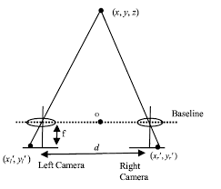
We don’t know the coordinate z of the point, but we do know where it gets projected on the plane of each camera. This gives us a ray starting at the plane of each camera with known angles. We also know the distance between the two projection points. What remain is determining where the two rays intersect.

It’s worth noting that to compute the ray’s angle we need to know the intrinsics of the camera, and specifically the focal length

Stereo vision is intuitive and simple. Image sensors are getting cheaper while resolution is going up. And, stereo vision has a lot in common with human vision, which means our systems can see exactly when people expect to see. And finally, stereo systems are passive — they don’t emit a signal into the environment — which makes them easier to build and energetically efficient.

But, stereo system isn’t a silver bullet. First, matching points/features between the two views can be computationally expensive and not very reliable. Second, some surfaces either don’t have features (white walls, shiny silver spoon, …) or have many features that are indistinguishable from each other. And finally, stereo doesn’t work when it’s too dark or too bright.

Structure from Motion

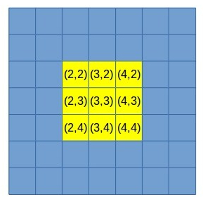
Structure from motion replace the fixed second camera in the stereo design with a single moving camera. The idea here is that as the camera is moving around the world, we can use views from two different perspectives to reconstruct depth much like we did in the stereo case.

Now’s a great time to say: “wait what?! didn’t you say stereo requires knowledge of the extrinsics?”. Great question! Structure from motion is more difficult in that we not only want to determine the depth of a point, but we also need to compute the camera motion. And no, it’s not an impossible problem to solve.

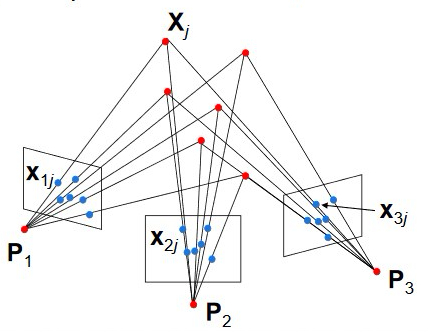
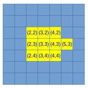
The key realization is that as the camera is moving, we can try to match many points between two views, not just one. We can assume that most points are part of the static environment (ie. not moving as well). Our camera motion model therefore must provide a consistent explanation for all points. Furthermore, with structure from motion we can easily obtain multiple perspectives (not just two like stereo).

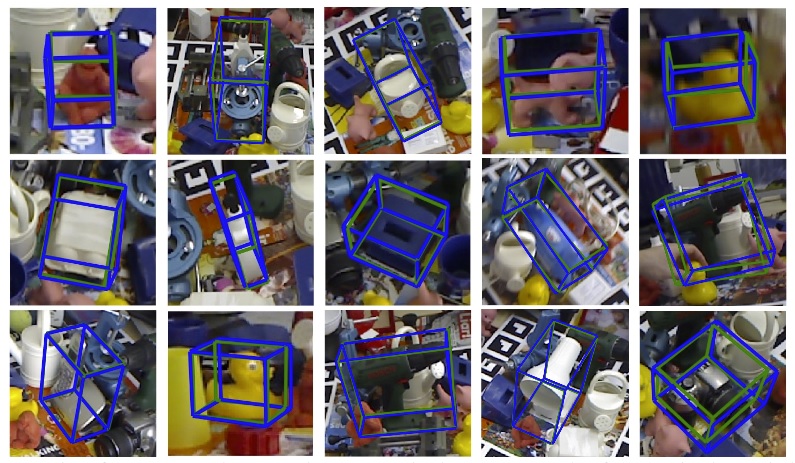
Structure from motion can be understood as a large optimization problem where we have N points in k frames and we’re trying to determine 6*(k-1) camera motion parameters and N depth values for our points from N*k observations. It’s easy to see how with enough points this problem quickly becomes over constrained and therefore very robust. For example, in the above image N=6 and k=3: we need to solve a system of 18 equations with 18 unknown.

The key advantages of structure from motion vs. stereo include simple hardware (just one camera), simple calibration (we only need intrinsics), and simple point matching (because we can rely on tracking frame-to-frame).

There are two main disadvantages. First, structure from motion is more complex mathematically. Second, structure from motion provides us a 3D reconstruction up to a scaling parameter. That is, we can always multiply the depth of all our points by some number and similarly multiply the camera’s motion and everything remains consistent. In stereo, this scaling ambiguity is solved through calibration: we know the baseline between the two cameras.

Structure from motion is typically solved as either an optimization problem (eg. bundle adjustment) or a filtering problem (eg. extended Kalman filter). It’s also quite common to mix the two: use bundle adjustment at a lower frequency and the Kalman filter at the measurement frequency (high).

 

3D Sensors

There are several technologies that try to measure depth directly. In contrast with the above methods, the goal is to recover depth from a single frame. Let’s discuss the most prominent technologies:

Active Stereo

We already know the advantages and disadvantages of stereoscopic vision. But what if our hardware could make some disadvantages go away?

In active stereo systems such as https://realsense.intel.com/stereo/ a noisy infra red pattern is projected on the environment. The system doesn’t know anything about the pattern, but its existence creates lots of features for stereo matching.

In addition, stereo matching is computed in hardware, making it faster and eliminates the processing burden on the host.

However, as its name implies, active stereo is an active sensor. Projecting the IR pattern requires additional power and imposes limitations on range. The addition of a projector also makes the system more complex and expensive to manufacture.

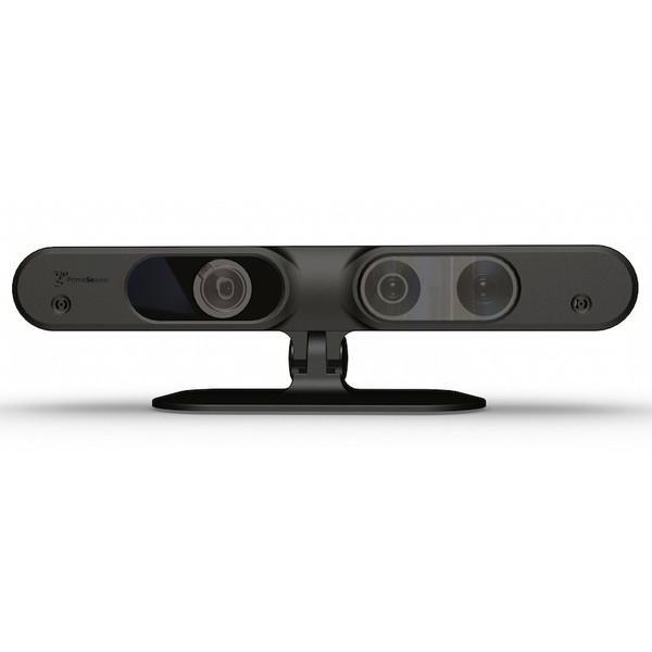
Structured Light

Structured light shares some similarities with active stereo. Here too a pattern is projected. However, in structured light a known pattern is projected onto the scene. Knowledge of how the pattern deforms when hitting surfaces enables depth reconstruction.

Typical structured light sensors (eg. PrimtSense) project infra red light and have no impact on the visible range. That is, humans cannot see the pattern, and other computer vision tasks are not impacted.

The advantages of structured light are that depth can be computed in a single frame using only one camera. The known pattern enable algorithmic shortcuts and results in accuracy and precise depth reconstruction.

Structured light, however, has some disadvantages: the system complexity increases because of the projector, computation is expensive and typically requires hardware acceleration, and infra red interference is possible.

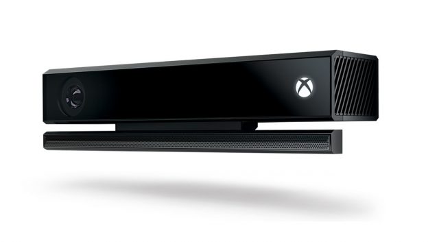
Time of Flight

Time of flight sensors derive their name from the physics behind the device. It relies on the known time it takes an infrared beam to travel a distance through a known medium (eg. air). The sensor emits a light beam and measures the time it takes for the light to return to the sensor from different surfaces in the scene.

Kinect One is an example of such sensor:

Time of Flight sensors are more expensive to manufacture and require careful calibration. They also have a higher power consumption compared to the other technologies.

However, time of flight sensors do all depth computation on chip. That is, every pixel measures the time of flight and returns a computed depth. There is practically no computational impact on the host system.

Summary

We reviewed different technologies for depth reconstruction. It’s obvious that each has advantages and disadvantages. Ultimately, if you are designing a system requiring depth, you’re going to have to make the right trade-offs for your setup.

A typical set of parameters to consider when choosing your solution is SWaP-C (Size, Weight, Power and Cost). Early on, it’s often better to choose a simple HW solution that requires significant computation and power. As your algorithmic solution stabilizes, it is easy to correct SWaP-C later on with dedicated hardware.

Where’s my point?

A reoccurring problem in computer vision has to do with finding the precise location of an object in the image. In this post, I want to discuss specifically the problem of finding the location of a blob or a point in an image. This is what you’d get when a light source is imaged.

Finding the center of the blob is a question I love asking in job interviews. It’s simple, can be solved with good intuition and without prior knowledge, and it shows a lot about how one grasps the process of image formation.

What’s a blob?

A blob is what’s formed on an image plane when imaging a light source. For instance, here’s how you might imagine a set of LEDs would appear in an image:

This is interesting problem because if we know the location of the center of each blob, and if we know the 3D pattern that generated it (eg. the 3D shape of the LED array) then we can reconstruct its position in 3D space.

There are many possible approaches here. Most of them are either too expensive computationally, unnecessarily complex or plainly inaccurate. Let’s discuss a few:

I) Averaging

This one is rather simple. We take all the pixels associated with a blob and find their average. Here are two examples:

Computing the average of all pixels above would give us x=3 and y=3 as the sum of all x coordinates and all y coordinates is 27 and there are 9 pixels.

Here, however, the average is different. Now the average x is 3.2 and the average y is still 3. This isn’t surprising — the center is shifting to the right because of the additional pixel.

This computation is simple and require very little computation. However, it’s obviously not very precise. We can easily see that our average is in the space of 1/2 pixel — the center either lands on a pixel center or its edge (between two pixels). This is terrible accuracy for 3D reconstruction (unless you have a super narrow field of view and/or extremely high resolution image sensor).

But wait, it gets worse. This method doesn’t take into account the brightness of pixels. For example, imagine pixel (5,3) above was extremely dim. So dim, in fact, that it would be just on the threshold of our image sensor. The result will be that the pixel would appear or disappear in consecutive frames due to image noise. The center of the blob will be greatly effected by this phenomena. Not good.

II) Circle Fit

How about fitting a circle to the blob? It seems like this would give us much higher precision and aren’t circles pretty robust to noise?

Well yes in theory but not so much in practice.

First, let’s consider the image of even a really small light source. The light source isn’t going to be a point source in practice. We can imagine it has some small circular shape. But, when that light source gets projected onto the image plane, the result is an ellipse and not a circle. Fitting an ellipse is much more complex and less robust than circle fit.

Second, the image formation process is unlikely to result in pixels that are all saturated. We are going to get shades of white as the distance from the true center increases. Here’s an example:

As can be seen in the image, pixels have less brightness when further out from the blob center. In fact, pixels at the edge of the blob might not always pass the sensor’s threshold and remain black. These pixels are going to have a significant impact on the fit.

And finally, in many cases blobs are going to be pretty small. Circle fit is much less robust with fewer pixels.

Weighted Average

A weighted average is almost as simple as the averaging method discussed above. However, it takes into account the strength of the signal in each pixel and it doesn’t assume the projected shape is a circle. Weighted average takes the brightness level of each pixel, and uses it as a weight for the average.

Now, imagine the 2nd example above, where all pixels have brightness level of 255, except for pixel (5,3) that is very dim, say brightness level of 10. Now, our weighted average will yield: x = 3.008 while y remains 3. This makes perfect sense: the dim pixel is pulling the center only slightly towards it. If that pixel was brighter, the pull would be stronger and the computed center will shift towards it.

Weighted average is also a great way to eliminate noise in the image. It’s simple, precise and much more robust.

Summary

I’ve used this method to solve multiple computer vision problems over time. Check out my patents page. Some of them use a version of this technique.