I developed the original position tracking for the Oculus Rift headset and controllers.
In this post, I will discuss why position tracking is important for Virtual Reality and how we realized it at Oculus.
What is Position Tracking?
Position tracking in the context of VR is about tracking the user’s head motion in 6D. That is, we want to know the user’s head position and orientation. Ultimately, we will expand this requirement to tracking other objects / devices such as controllers or hands. But for now, I’ll focus on head motion.
Tracking the head let’s us render the right content for the user. For instance, as you move your head forward, you expect the 3D virtual world to change: objects will get closer to you, certain object will go out of the field of view, etc. Similarly, when you turn around, you expect to see what was previously behind you.
Virtual reality can cause motion sickness. If the position and orientation updates are wrong, shaky or just imprecise, our brain will sense the conflict between proprioception and vision — we know how the head, neck and body is moving, and we know what we expect to see, the mismatch causes discomfort.
To give you a sense of the requirements: we’re looking for a mean precision of about 0.05[mm] and a latency of about 1[ms]. In the case of a consumer electronics device, we also want to system cost to be low in $ and computation.
Note: the following assumes tracking of a single headset using a single camera. Mathematically, using stereo is easier. However, the associated cost in manufacturing and calibration are significant.
Basic Math
We can compute the pose of an object if we know its structure. In fact, we need as few as 3 points to compute a 6D pose:
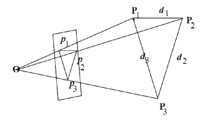
If we know the distance between P1, P2 and P3 in metric units and the camera properties (intrinsics), we can compute the pose of the object (P1,P2,P3) that creates the projection (p1,p2,p3).
There are just two hurdles:
(1) we need to be able to tell which point P(i) corresponds to a projected point p(j)
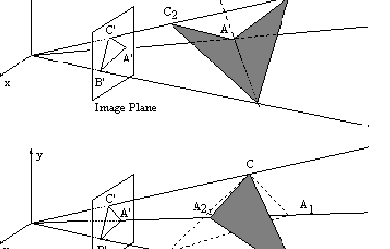
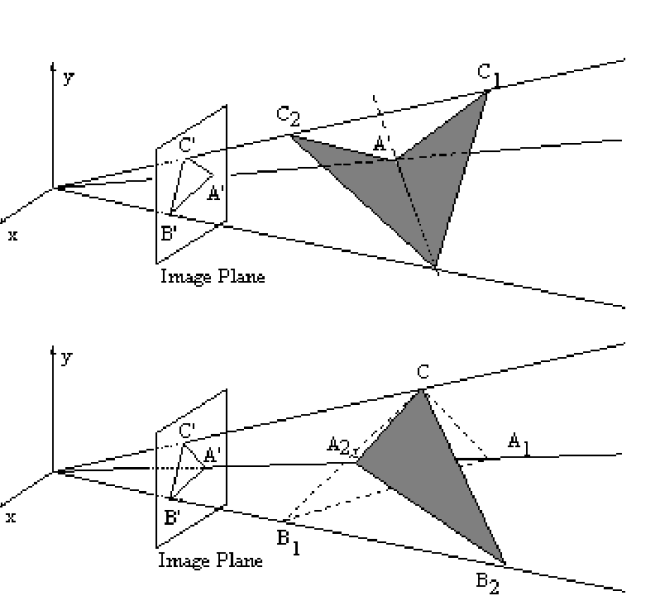
(2) in the above formulation, there can actually be more than one solution (pose) that creates the same projection
Here’s an illustration of #2:
ID’ing points
There are many ways to solve #1. For instance, we could color code the points so they are easy to identify. At Oculus we created the points using infra red LEDs on the headset. We used modulation — each LED switched between high and low — to create a unique sequence.
Later on, we were able to make the computation efficient enough that we didn’t need modulation. But that’s for another post 🙂
Dealing with multiple solutions
There are two primary ways to handle multiple solutions. First, we have many LEDs on the headset. This means that we can create many pose theories for subsets of 3 points. We expect the right pose to explain all of them. Second, we are going to track the pose of the headset over time — the wrong solution will make tracking break in the next few frames because while the right answer will change smoothly from frame to frame, the alternative pose solution will jump around erratically.
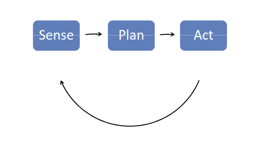
Tracking
Many problems in computer vision can be solved by either tracking or re-identification. Simply put, you can either use the temporal correlation between solutions or recompute the solution from scratch every frame.
Usually, taking advantage of the temporal correlation leads to significant computational savings and robustness to noise. However, the downside is that we end up with a more complex software: we use a “from scratch” solution for the first frame and a tracking solution for the following frames. When you design a real time computer vision system, you often have to balance the trade-off between the two options.
The Oculus’ position tracking solution uses tracking. We compute the pose for frame i as discussed above, and then track the pose of the headset in the following frames. When we compute the pose in frame n, we know where the headset was in frame n-1 and n-2. This means that not only we have a good guess for the solution (close to where it was in the previous frame), but we also know the linear and angular velocities of the headset.
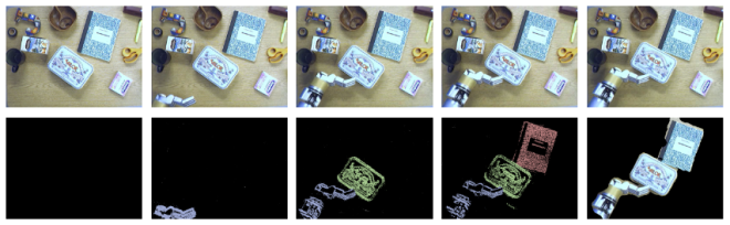
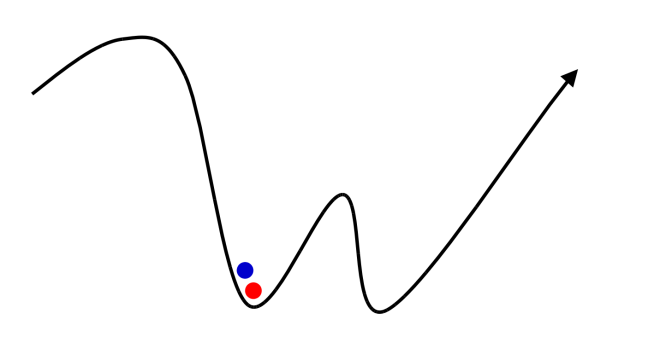
The following illustration shows the process of refining the pose of the headset based on temporal correlation. We can make a guess for the pose of the headset (the blue point). We then compute where the projected LEDs should be in the image given that pose. Of course, there are going to be some errors — we can now adjust the pose locally to get the red solution below (the local minima).
Latency
So far so good — we have a clean solution to compute the pose of the headset over time using only vision data. Unfortunately, a reasonable camera runs at about 30[fps]. This means that we’re going to get pose measurements every 33[ms]. This is very far from the requirement of 1[ms] of latency…
Let me introduce you to the IMU (Inertial Measurement Unit). It’s a cheap little device that is part of every cellphone and tablet. It’s typically being used to determine the orientation of your phone. The IMU measures the linear acceleration and angular velocity. And, a typical IMU works at about 1[KHz].
Our next task, therefore, is to use the IMU together with vision observations to get pose estimation at 1[KHz]. This will satisfy our latency requirements.
Complementary Filter
The complementary filter is a well known method for integrating multiple sources of information. We are going to use it to both filter IMU measurements to track the orientation of the headset, and to fuse together vision and IMU data to get full 6D pose.
IMU: orientation
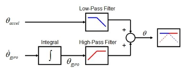
To compute the orientation of the headset from IMU measurements we need to know the direction of gravity. We can compute that from the acceleration measurements. The above figure shows we can do that by low-pass filtering the acceleration vector. As the headset moves around, the only constant acceleration the IMU senses is going to be gravity.
orientation = (orientation + gyro * dt) * (1 – gain) + accelerometer * gain
With knowledge of gravity, we can lock the orientation along two dimensions: tilt and roll. We can also estimate the change in yaw, but this degree of freedom is subject to drift and cannot be corrected with gravity. Fortunately, yaw drift is slow and can be corrected with vision measurements.
IMU: full 6D pose
The final step in our system integrates pose computed from the camera (vision) at a low frequency with IMU measurements at a high frequency.
err = camera_position – filter_position
filter_position += velocity * dt + err * gain1
velocity += (accelerometer + bias) * dt + err * gain2
bias += err * gain3
Summary
Now we have a fully integrated system that takes advantage of the advantages of the camera (position and no drift in yaw) and the IMU (high frequency orientation and knowledge of gravity).
The complementary filter is a simple solution that provides as with smooth pose tracking at a very low latency and with minimal computational cost.
Here’s a video of a presentation I gave together with Michael Abrash about VR at Carnegie Mellon University (CMU). In my part, I cover the position tracking system design.